Running the Simulation Software


  At the current time, executable files are only available for Linux operating environments and are located on the GitHub page for Geno-Diver. It has also been tested on a MAC operating environment and the manual describes how to compile the program. To run the program place, "GenoDiver", "macs" and "msformatter" executable files in the folder where the program will run. Before running the program, the file permissions need to be checked. After verifying the permissions, a parameter file, outlined below, will need to be generated and placed in the same folder as the previous three executable files. A parameter file can be generated using any text editor.

  The simulation program reads the parameter file by searching for keywords that are capitalized and followed by a colon. Therefore any phrase that does not meet the search criteria is ignored when initializing parameters within the program. Also, if you want to comment out a parameter just add "!!" within the key word and the program will skip over it. For example to skip over the "SEED" parameter just replace it with "SE!!ED" and it won't recognize the parameter any more.

−−−−−−−| Running the Program Example |−−−−−−−
−| General |−
START: sequence
SEED: 1500
−| Genome & Marker |−
CHR: 3
CHR_LENGTH: 150 150 150
NUM_MARK: 4000 4000 4000
QTL: 150 150 150
−| Population |−
FOUNDER_Effective_Size: Ne70
MALE_FEMALE_FOUNDER: 50 400 random 3
VARIANCE_A: 0.10
−| Selection |−
GENERATIONS: 15
INDIVIDUALS: 50 0.2 400 0.2
PROGENY: 1
SELECTION: ebv high
EBV_METHOD: pblup
CULLING: ebv 5
-| Mating |-
MATING: random125 simu_anneal

Parameter File Summary
  Sequence information is generated for three chromosomes with a length of 150 Megabases (Mb). The simulated genome has a high degree of short- range LD (Ne70). The SNP panel contains 12,000 markers (i.e. 4,000 mark- ers per chromosome). For each chromosome, 150 randomly placed QTL and zero FTL mutations were generated. The quantitative trait simulated has a narrow sense heritability of 0.10 and only additive effects are generated (i.e. no dominance). The phenotypic variance is by default set at 1.0, and therefore the residual variance is 0.90. The founder population consisted of 50 males and 400 females. For each generation, a total of 50 males and 400 females are in the population. Random selecton of progeny and culling of parents was conducted for 3 generations in order to build up the pedigree. A total of 10 and 80 (0.2 replacement rate) male and female parents, re- spectively, are culled and replaced by new progeny each generation. After 3 generations, animals with a high EBV are selected or culled each gener- ation. Fifteen generations are simulated. The EBV are estimated using an animal model with a pedigree-based relationship matrix. Each mating pair produced one progeny. Parents with a pedigree-based relationships greater than 0.125 were avoided, and this was optimized based on the simulated annealing method.

  To run the program type “./GenoDiver” and the name of your parameter file. For example, if the parameter file is named “parameterfile”, the program is run by typing in “./GenoDiver parameterfile”. During the simulation, the program outputs minimal comments on the progress. A more thorough description of the program's status is printed to the log file (i.e. “log_file.txt”).

  After the program has finished it is a strongly recommended to check the parameters initialized at the top of the log file (i.e. "log_file.txt") within the output folder. The log file contains a large amount of information and is a great tool to ensure that the parameters and outcome of the simulation is what is intended. If the program is not running correctly the log file should provide knowledge on why and where the simulation crashed or exited.

  The files are by default placed in the "GenoDiverFiles" directory. If the "OUTPUTFOLDER" option is utilized, the files will be placed in the user-specified directory. Below is a screenshot of the files that are generated from the simulation software based on the parameter file outlined above.

  A number of files are generated, but only a few are needed to generate summary statistics on the simulation program and include:
  • Master_DataFrame: File with phenotype, inbreeding and pedigree information across all animals.
  • Master_Genotypes.gz: File with genotype information for each animal.
  • QTL_new_old_Class: File with information for each QTL/FTL mutation.
  • Marker_Map: Location of markers.
  • Summary_Statistics_DataFrame_Performance: Statistics by generation for performance metrics.
  • Summary_Statistics_DataFrame_Inbreeding: Statistics by generation for inbreeding metrics.
  • Summary_Statistics_QTL: Statistics by generation for QTL/FTL metrics.
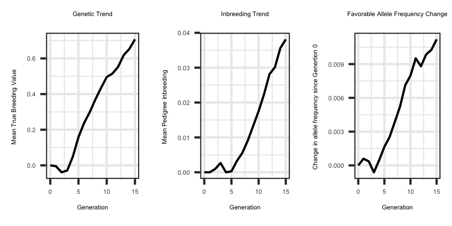
  Utilizing the R code outlined below the following plots were generated from the output files. The following example utilizes traditional pedigree information when predicting breeding values for individuals. To test the impact of genomic information on the plots outlined below change the EBV_METHOD to 'gblup' and use the R code below to see the difference.

R-Code
rm(list = ls()); gc()
library(ggplot2); library(tidyverse)
## Change
setwd("/Users/jeremyhoward/Desktop/C++Code/18_GenoDiver_V3/GenoDiverFiles/")
#############################
## Plot True Genetic Value ##
#############################
df <- read_table2(file="Summary_Statistics_DataFrame_Performance",col_names = TRUE,col_type = "dcccccc") %>%
mutate(.,tbv = as.numeric(matrix(unlist(strsplit(tbv, "[()]")), ncol = 2, byrow = TRUE)[, 1])) %>%
select(Generation,tbv)

ggplot(df, aes(x = Generation, y = tbv)) + geom_line(size = 1) + ggtitle("Genetic Trend") + theme_bw() +
theme(plot.title = element_text(hjust = 0.5)) + ylab("Mean True Breeding Value ")
##############################
## Plot Pedigree Inbreeding ##
##############################
df <- read_table2(file="Summary_Statistics_DataFrame_Inbreeding",col_names = TRUE,col_type = "dcccccccccccccc") %>%
mutate(.,ped_f = as.numeric(matrix(unlist(strsplit(ped_f, "[()]")), ncol = 2, byrow = TRUE)[, 1])) %>%
select(Generation,ped_f)

ggplot(df, aes(x = Generation, y = ped_f)) + geom_line(size = 1) + ggtitle("Inbreeding Trend") + theme_bw() +
theme(plot.title = element_text(hjust = 0.5)) + ylab("Mean Pedigree Inbreeding ") + xlab("Generation")
#############################
## Allele Frequency Change ##
#############################
df <- read_table2(file="QTL_new_old_Class",col_names = TRUE,col_type = "dcccccc")
## split apart frequencies ##
freq <- matrix(unlist(strsplit(df$Freq, "_")), ncol = 16, byrow = TRUE)
freq <- apply(freq, 2, as.numeric)
## y axis is in terms of change in the favorable direction ##
## grab ones with a positive effect and subtract of initial value #
X <- which(df$Additive_Selective > 0)
freq[X, ] <- freq[X, ] - freq[X, 1]
## grab ones with a negative effect and subtract of initial value #
X <- which(df$Additive_Selective < 0)
freq[X, ] <- (freq[X, 1] - freq[X, ])
## get mean by generation
plotdf <- data.frame(cbind(c(0:15), colMeans(freq)))
names(plotdf) <- c("gen", "freq")

ggplot(plotdf, aes(x = gen, y = freq)) + geom_line(size = 1.0) + ggtitle("Favorable Allele Frequency Change") + theme_bw() +
theme(plot.title = element_text(hjust = 0.5)) + ylab("Change in allele frequency since Genertion 0 ") +
xlab("Generation")