The parameter file below illustrates how to simulate a fitness trait only. When simulating a fitness trait it is important to
ensure that you have enough founder individuals because a portion will not make it to breeding age. Therefore, an extra 140 males and
200 females were added to the founder population to ensure enough individuals are available to generate the breeding population. This
will also impact the replacement rate because if enough progeny aren't available to remain at the chosen male and female population size
the simulation will exit. A full description of how the fitness value of an individual impacts its ability to make it to breeding age
is described in the "QTL/FTL Distribution Parameters" link.
−−−−−−−| Simulating a Fitness Trait |−−−−−−−
−| General |−
START: sequence
SEED: 1500
−| Genome & Marker |−
CHR: 3
CHR_LENGTH: 150 150 150
NUM_MARK: 4000 4000 4000
QTL: 0 0 0
FIT_LETHAL: 50 50 50
FIT_SUBLETHAL: 50 50 50
−| Population |−
FOUNDER_Effective_Size: 250
MALE_FEMALE_FOUNDER: 150 600 random 0
VARIANCE_A: 0.0
−| Selection |−
GENERATIONS: 25
INDIVIDUALS: 10 0.2 400 0.2
PROGENY: 1
SELECTION: random high
CULLING: random 10
-| Mating |-
MATING: random
-| OUTPUT OPTIONS |-
GENOTYPES: no
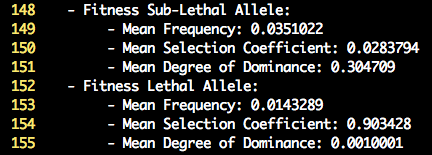
Inspection of the log file will provide summary statistics on the mean selection coefficients and degree of dominance for the lethal and sub-lethal
fitness effect along with their associated frequency. The default settings for the lethal mutations result in a high selection coefficient (0.90) and very little
dominance (0.001). Therefore the heterozygote is normal, while the unfavorable homozygote has a low fitness value. The settings for the sub-lethal mutations result in a
lower selection coefficient (0.03) and moderate degree of dominance (0.30). Therefore the heterozygote now has a reduced fitness value compared to the fittest homozygote.
Lastly, the mean allele frequency of the unfavorable allele is higher for sub-lethal compared to lethals. Below is a screenshot of the lines in the log file that display
the summary statistics.
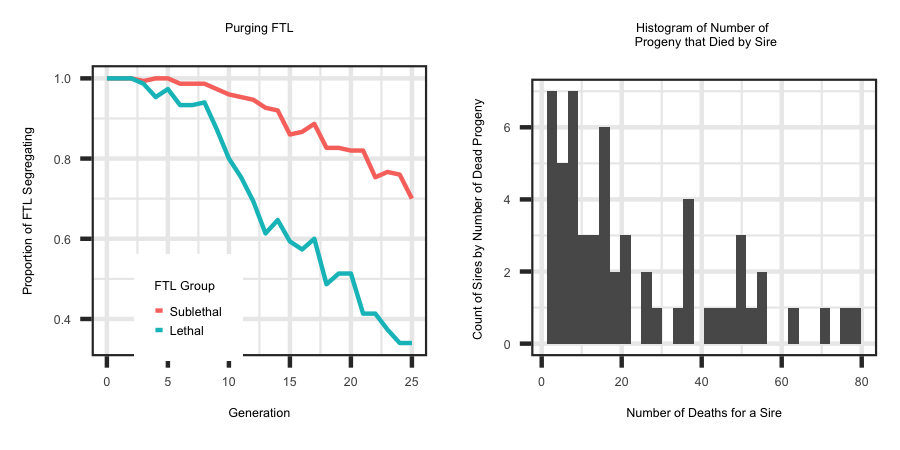
When a fitness trait is simulated, the animals that died due to fitness are placed in the "Low_Fitness" along with summary statistics for the respective animals.
Utilizing the R code outlined below the following plots were generated to illustrate the type of information in the "Low_Fitness" file.
R-Code
rm(list=ls()); gc()
library(ggplot2); library(tidyverse)
setwd("/Users/jeremyhoward/Desktop/C++Code/18_GenoDiver_V3/GenoDiverFiles/")
df <- read_table2(file="QTL_new_old_Class",col_names = TRUE,col_type = "dcccccc")
freq <- matrix(unlist(strsplit(df$Freq, "_")), ncol = 26, byrow = TRUE)
freq <- apply(freq, 2, as.numeric)
X <- which(freq[,1] > 0.50)
freq[X, ] <- 1 - freq[X, ]
freq <- ifelse(freq == 0.0, 0,1)
X <- which(df$Type == 5)
plotdf <- data.frame(Generation = c(0:25),
PropSegregating = colSums(freq[X, ]) / length(X),
Group = c(rep("Sublethal",26)))
X <- which(df$Type == 4)
plotdfa <- data.frame(Generation = c(0:25),
PropSegregating = colSums(freq[X, ]) / length(X),
Group = c(rep("Lethal",26)))
plotdf <- rbind(plotdf,plotdfa); rm(X,plotdfa)
ggplot(plotdf, aes(x = Generation, y = PropSegregating,group=Group, colour = Group)) + geom_line() + theme_bw() +
labs(title = "Purging FTL", x = "Generation", y = "Proportion of FTL Segregating") +
scale_colour_discrete(name ="FTL Group") + theme(plot.title = element_text(hjust = 0.5), legend.position="bottom")
df <- read_table2(file="Low_Fitness",col_names = TRUE,col_type = "iiiddddiiiiddcddd")
SireDeath <- aggregate(TGV ~ Sire, data=df,FUN=length)
SireDeath <- SireDeath[which(SireDeath$Sire != 0), ]
SireDeath <- SireDeath[order(-SireDeath$TGV), ]
ggplot(data=SireDeath, aes(SireDeath$TGV)) + geom_histogram() + theme_bw() +
ylab ("Count of Sires by Number of Dead Progeny ") + xlab ("Number of Deaths for a Sire") + theme_bw()+
ggtitle("Histogram of Number of \n Progeny that Died by Sire") + theme(plot.title = element_text(hjust = 0.5))


