The parameter file outlined below illustrates how to simulate a quantitative trait that has a proportion (i.e. 50%) of the quantitative trait loci (QTL) also having
a fitness effect. The relationship between the QTL with a fitness effect has a positive correlation of 0.20, but the two traits are antagonistic based on the way the fitness
value of a loci is parameterized. High selection coefficients (s) result in the unfavorable homozygote genotype to be less fit and is described in detail in the 'QTL/FTL
Distributions' link. As outlined in the previous example, it is important to add a few extra animals in the founder population since a portion will die. If the number of male
or female founder animals is smaller than the population size it will exit out of the program. Therefore, careful consideration of the number and magnitude of fitness effects
along with the number of progeny produced per mating pair needs to be carefully considered when constructing the simulation design.
−−−−−−−| Quantitative and Fitness Trait |−−−−−−−
−| General |−
START: sequence
SEED: 1501
−| Genome & Marker |−
CHR: 3
CHR_LENGTH: 150 150 150
NUM_MARK: 4000 4000 4000
QTL: 150 150 150
FIT_LETHAL: 15 15 15
FIT_SUBLETHAL: 100 100 100
−| Population |−
FOUNDER_Effective_Size: Ne70
MALE_FEMALE_FOUNDER: 100 400 random 3
VARIANCE_A: 0.20
VARIANCE_D: 0.05
COVAR: 0.5 0.2
−| Selection |−
GENERATIONS: 20
INDIVIDUALS: 50 0.2 250 0.2
PROGENY: 1
SELECTION: ebv high
EBV_METHOD: pblup
CULLING: ebv 5
-| Mating |-
MATING: random
Inspection of the log file will provide summary statistics on the mean selection coefficients and degree of dominance for the lethal and sub-lethal
fitness effect along with their associated frequency. The default settings for the lethal mutations result in a high selection coefficient (0.90) and very little
dominance (0.001). Therefore the heterozygote is normal, while the unfavorable homozygote has a low fitness value. The settings for the sub-lethal mutations result in a
lower selection coefficient (0.02) and moderate degree of dominance (0.30). Therefore the heterozygote now has a reduced fitness value compared to the fittest homozygote.
Lastly, the mean allele frequency of the unfavorable allele is higher for sub-lethal compared to lethals. Below is a screenshot of the lines in the log file that display
the summary statistics.
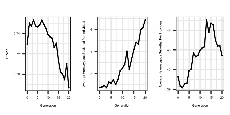
Utilizing the R code outlined below the following plots were generated from the output files.
R-Code
rm(list=ls()); gc()
library(ggplot2); library(tidyverse)
setwd("/Users/jeremyhoward/Desktop/C++Code/18_GenoDiver_V3/GenoDiverFiles/")
df <- read_table2(file="Summary_Statistics_DataFrame_Inbreeding",col_names = TRUE,col_type = "dcccccccccccccc") %>%
mutate(fitness = as.numeric(matrix(unlist(strsplit(fitness, "[()]")), ncol = 2, byrow = TRUE)[, 1]),
homosublethal = as.numeric(matrix(unlist(strsplit(homozysublethal, "[()]")), ncol = 2, byrow = TRUE)[, 1]),
hetezsublethal = as.numeric(matrix(unlist(strsplit(hetezsublethal, "[()]")), ncol = 2, byrow = TRUE)[, 1])) %>%
select(Generation,fitness,homosublethal,hetezsublethal)
ggplot(df, aes(x=Generation, y = fitness)) + geom_point(size = 3) + geom_line()
labs(title = "", x = "Generation", y = "Fitness") + theme_bw() +
ggplot(df, aes(x=Generation, y = homosublethal)) + geom_point(size = 3) + geom_line()
labs(title = "", x = "Generation", y = "Average Homozygous Sublethal Per Individual") + theme_bw() +
ggplot(df, aes(x=Generation, y = hetezsublethal)) + geom_point(size = 3) + geom_line()
labs(title = "", x = "Generation", y = "Average Heterozygous Sublethal Per Individual") + theme_bw()


