A bash script is outlined below that illustrates how to loop through different simulation scenarios. The following script may take
a couple of hours to finish depending on the computing environment. The difference between the scenarios is how estimated breeding values
(EBV) are estimated across individuals. The four methods to predict EBV are: a pedigree-based best linear unbiased prediction (BLUP) animal
model, a genomic-based BLUP animal model, a run-of-homozygosity-based BLUP animal model and a Bayesian spike and slab marker effects model
(BayesC). All three scenarios utilize the same founder sequence, which is generated by first using the 'sequence' option for the "START"
parameter and then the remaining scenarios use the 'founder' option for the "START" parameter. In order to generate multiple replicates
within each scenario, the "NREP" parameter is utilized and 15 replicates were generated within each scenario. The replicates are saved
within the "GenoDiverFiles" directory for each scenario. If the directory isn't renamed, the next scenario will replace the files. Therefore,
after a scenario is done the directory is renamed within the bash script.
Outlined below is a more detailed explanation of the major differences in how EBVS are calculated across the
different scenarios:
- pblup: The EBV are estimated based on a relationship matrix derived from pedigree information. All animals
are utilized when generating the relationship matrix.
- gblup: The EBV are estimated based on a relationship matrix derived from genomic information (G). When
generating the relationship matrix all animals are utilized along with all of the markers. Therefore, the assumption is that all markers
have an impact on the phenotype. Furthermore, allele frequencies utilized to construct G are estimated from the founder population.
- rohblup: The EBV are estimated based on a relationship matrix derived from runs-of-homozygosity (ROH). When
generating the relationship matrix all animals are utilized along with all of the markers. Therefore, the assumption is that all markers
have an impact on the phenotype.
- bayes: The EBV are estimated based on bayesian marker effects model, which estimates the effect of each
marker utilizing an MCMC approach. An animals EBV is generated by the summation of an animals genotype times the estimated marker effect
across all markers. When the 'bayes' option is specified, the "BAYESOPTIONS" parameter must be included in the parameter file. The model
used is referred to as BayesC, which is a spike and slab marker effects model. The 5 values after specifying which type of bayesian model
to implement refers to how many iterations to run the MCMC chain and the thinning rate. The first time the BayesC model is implemented
(i.e. Generation 6), a total of 10,000 MCMC iterations are generated with the first 2,000 discarded as burn-in. The following generations
then use the marker effects from the previous generation as starting values and a total of 6,000 MCMC iterations are generated with the
first 1,000 discarded as burn-in. Lastly, a thinning rate of 5 is utilized. In BayesC it assumed only a proportion of the markers have
a non-null effect, while the remaining don't have an effect. In this case we fixed the proportion and we assumed 10 % of the markers
have an effect. One of the downfalls with MCMC sampling is that it does increase the computation time. Therefore you will notice that
when using the bayes options the computation time will dramatically increase.
The important files are saved within the renamed replicate folder within each scenario. The replicate number is appended to the file name.
The bash script above renames the replicate directories to "reps_pblup", "reps_gblup", "reps_rohblup" and "reps_bayesC" for the pblup, gblup, rohblup
and bayes EBV estimation scenarios, respectively. A screenshot of the files within the "GenoDiverFiles" is below. The directories are in blue and
the files are in white.
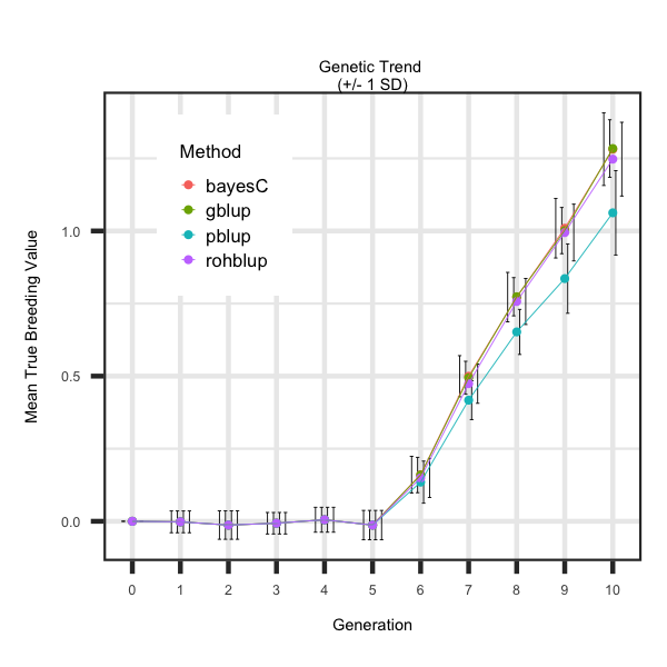
Utilizing the R code outlined below the following plot was generated to illustrate how to loop through each scenario and generate plots
that describe the impact of EBV estimation method on the genetic trend.
R-Code
rm(list=ls()); gc()
library(ggplot2); library(tidyverse)
wd <- "/Users/jeremyhoward/Documents/39_GenoDiver_C++Code/WebsiteExamples/Example12/"
scen <- c("reps_pblup","reps_gblup","reps_rohblup","reps_bayesC")
reps <- c(1500:1514)
for(i in 1:length(scen))
{
for(j in 1:length(reps))
{
filename <- paste(wd,scen[i],"/Summary_Statistics_DataFrame_Performance_",reps[j],sep="")
df <- read_table2(file=filename,col_names = TRUE,col_type = "dcccccc") %>%
mutate(tgv = as.numeric(matrix(unlist(strsplit(tgv, "[()]")), ncol = 2, byrow = TRUE)[, 1]),
Method = unlist(strsplit(scen[i],"_"))[2], Rep = reps[j]) %>%
select(Generation,Method,Rep,tgv)
if(j == 1 & i == 1){summarytable <- df}
if(j > 1 | i > 1){summarytable <- rbind(summarytable,df);}
}
}
means <- aggregate(tgv ~ Generation + Method, data=summarytable,FUN=mean)
sds <- aggregate(tgv ~ Generation + Method, data=summarytable,FUN=sd)
plotdf <- cbind(means,sds[,3]); rm(means,sds)
names(plotdf) <- c("Generation","Method","Mean","SD")
pd <- position_dodge(0.20)
ggplot(plotdf, aes(x=as.factor(Generation), y=Mean, group=Method, colour=Method)) +
geom_errorbar(aes(ymin=Mean-SD, ymax=Mean+SD), colour="black", width=.4, size = 0.5, position=pd) +
geom_point(size=2.0) + geom_line(size=0.50) + theme_bw() +
labs(title = "Genetic Trend \n(+/- 1 SD)", x = "Generation", y = "Mean True Breeding Value") +
theme(plot.title = element_text(size = 16,hjust = 0.5),axis.title = element_text(size = 12),
legend.position="bottom",axis.text=element_text(size=10))


