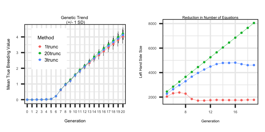
Similar to the previous example, a bash script is outlined below that illustrates how to reduce the memory requirements by truncating
animals born 'n' generations ago. This is especially useful if you want to simulate a large number of generations (25+) and as outlined below
truncating the data to only include recently born animals does not have a large impact on the genetic trend across generations. To truncate animals for BLUP
based ebv prediction the "BLUP_OPTIONS" parameter needs to be included and the first option specifies how many generations back from the current
group of selection candidates you want to go. For example, if a value of 1 is specified the selection candidate’s parents and the associated parents
progeny will only be included in the analysis. The default value is the number of generations simulated (i.e. all animals are used each generation).
The bash script outlined below uses the 'gblup' option to generate breeding values but either uses all the animals, 3 or 1 generations back from the
selection candidates to estimate breeding values. A total of 15 replicates were generated. After a scenario is done the directory where the replicates
are saved is renamed within the bash script.
Similar to Example 12, the important files are saved within the renamed replicate folder within each scenario. The replicate number is appended to the file name.
The bash script above renames the replicate directories to "reps_20trunc", "reps_3trunc" and "reps_1trunc" for the model that uses all animals, 3 generations back or
1 generation back, respectively.
Utilizing the R code outlined below the following plot was generated to illustrate how to loop through each scenario and generate plots
that describe the impact of truncating animals on the genetic trend and the reduction in the number of equations to solve. Also, within the R code
it illustrated how you can read in the log file and grab metrics across generations.
R-Code
rm(list=ls()); gc()
library(ggplot2); library(tidyverse)
wd <- "/Users/jeremyhoward/Documents/39_GenoDiver_C++Code/WebsiteExamples/Example13/"
scen <- c("reps_20trunc","reps_3trunc","reps_1trunc")
reps <- c(1500:1514)
for(i in 1:length(scen))
{
for(j in 1:length(reps))
{
filename <- paste(wd,scen[i],"/Summary_Statistics_DataFrame_Performance_",reps[j],sep="")
df <- read_table2(file=filename,col_names = TRUE,col_type = "dcccccc") %>%
mutate(tgv = as.numeric(matrix(unlist(strsplit(tgv, "[()]")), ncol = 2, byrow = TRUE)[, 1]),
Method = unlist(strsplit(scen[i],"_"))[2], Rep = reps[j]) %>%
select(Generation,Method,Rep,tgv)
if(j == 1 & i == 1){summarytable <- df}
if(j > 1 | i > 1){summarytable <- rbind(summarytable,df);}
}
}
means <- aggregate(tgv ~ Generation + Method, data=summarytable,FUN=mean)
sds <- aggregate(tgv ~ Generation + Method, data=summarytable,FUN=sd)
plotdf <- cbind(means,sds[,3]); rm(means,sds)
names(plotdf) <- c("Generation","Method","Mean","SD")
pd <- position_dodge(0.20)
ggplot(plotdf, aes(x=as.factor(Generation), y=Mean, group=Method, colour=Method)) +
geom_errorbar(aes(ymin=Mean-SD, ymax=Mean+SD), colour="black", width=.4, size = 0.5, position=pd) +
geom_point(size=2.0) + geom_line(size=0.50) + theme_bw() +
labs(title = "Genetic Trend \n(+/- 1 SD)", x = "Generation", y = "Mean True Breeding Value") +
theme(plot.title = element_text(size = 16,hjust = 0.5),axis.title = element_text(size = 12),
legend.position="bottom",axis.text=element_text(size=10))
for(i in 1:length(scen))
{
for(j in 1:length(reps))
{
filename <- paste(wd,scen[i],"/log_file_",reps[j],sep="")
df <- scan(file=filename,sep="\n",what=character(),quiet = TRUE);
tempa <- df[grep("Begin Generation",df)]; tempa <- tempa[6:length(tempa)-1]
tempa <- as.numeric(matrix(unlist(strsplit(tempa," ")),ncol = 5,byrow=TRUE)[ ,c(4)])
tempb <- df[grep("Size of Relationship Matrix",df)];
tempb <- unlist(strsplit(tempb," ")); tempb <- tempb[which(tempb != "")]
tempb <- matrix(tempb,ncol = 8,byrow=TRUE); tempb <- as.numeric(tempb[c(1:(nrow(tempb)-1)),c(6)]); tempb <- tempb+1;
df <- data.frame(cbind(tempa,tempb),stringsAsFactors = FALSE)
df$Method <- unlist(strsplit(scen[i],"_"))[2]
df$Rep <- reps[j];
names(df) <- c("Generation","LHS_Size","Method","Rep")
if(j == 1 & i == 1){summarytable <- df;}
if(j > 1 | i > 1){summarytable <- rbind(summarytable,df);}
}
}
summarytable$LHS_Size <- as.numeric(paste(summarytable$LHS_Size))
means <- aggregate(LHS_Size ~ Generation + Method, data=summarytable,FUN=mean)
sds <- aggregate(LHS_Size ~ Generation + Method, data=summarytable,FUN=sd)
plotdf <- cbind(means,sds[,3]); rm(means,sds)
names(plotdf) <- c("Generation","Method","Mean","SD")
pd <- position_dodge(0.5)
ggplot(plotdf, aes(x=Generation, y=Mean, colour=Method)) +
geom_errorbar(aes(ymin=Mean-SD, ymax=Mean+SD), colour="black", width=.4, size = 0.5, position=pd) +
geom_point(size=2.0) + geom_line(size=0.50) + theme_bw() +
labs(title = "Reduction in Number of Equations", x = "Generation", y = "Left Hand Side Size") +
theme(plot.title = element_text(size = 16,hjust = 0.5),axis.title = element_text(size = 12),
legend.position="bottom",axis.text=element_text(size=10))


