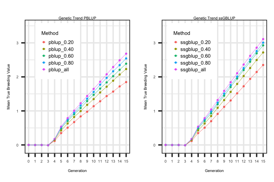
Similar to the previous examples, a bash script is outlined below that illustrates the impact of different phenotyping strategies on the
long term genetic trend when generating breeding values using either pedigree BLUP (pblup) or single step genomic BLUP (ssgblup). Within each
each breeding value method phenotypes on all or a random 80, 60, 40 or 20 percent of the selection candidates were collected. A total of
15 replicates were generated. After a scenario is done the directory where the replicates are saved is renamed within the bash script.
Similar to Example 6, the important files are saved within the renamed replicate folder within each scenario. The replicate number is appended to the file name.
Outlined below is a more detailed explanation of the major differences in the phenotyping scenarios:
- pheno_atselection: All selection candidates have phenotype information and they are utilized when ebv are being predicted.
- random_atselection: Only a certain percentage of the selection candidates have phenotype information and they are utilized when ebv are being predicted.
Utilizing the R code outlined below the following plot was generated to illustrate how to loop through each scenario and generate plots
that describe the impact of reducing the number of phenotypes that are collected on the true breeding value genetic trend for pblup and ssgblup
breeding value predictions.
R-Code
rm(list=ls()); gc()
library(ggplot2); library(tidyverse)
wd <- "/Users/jeremyhoward/Documents/39_GenoDiver_C++Code/WebsiteExamples/Example16/"
scen <- c("reps_pblup_0.20","reps_pblup_0.40","reps_pblup_0.60","reps_pblup_0.80","reps_pblup_all" ,"reps_ssgblup_0.20","reps_ssgblup_0.40","reps_ssgblup_0.60","reps_ssgblup_0.80","reps_ssgblup_all")
reps <- c(1500:1514)
for(i in 1:length(scen))
{
for(j in 1:length(reps))
{
filename <- paste(wd,scen[i],"/Summary_Statistics_DataFrame_Performance_",reps[j],sep="")
df <- read_table2(file=filename,col_names = TRUE,col_type = "dcccccc") %>%
mutate(tbv = as.numeric(matrix(unlist(strsplit(bv, "[()]")), ncol = 2, byrow = TRUE)[, 1]),
Method = paste(unlist(strsplit(scen[i],"_"))[2:length(unlist(strsplit(scen[i],"_")))],collapse = '_'),
Rep = reps[j]) %>%
select(Generation,Method,Rep,tbv)
if(j == 1 & i == 1){summarytable <- df}
if(j > 1 | i > 1){summarytable <- rbind(summarytable,df);}
}
}
means <- aggregate(tbv ~ Generation + Method, data=summarytable,FUN=mean)
sds <- aggregate(tbv ~ Generation + Method, data=summarytable,FUN=sd)
plotdf <- cbind(means,sds[,3]); rm(means,sds)
names(plotdf) <- c("Generation","Method","Mean","SD")
pd <- position_dodge(0.20)
plotdfa <- plotdf[which(plotdf$Method == "pblup_0.20" | plotdf$Method == "pblup_0.40" | plotdf$Method == "pblup_0.60" | plotdf$Method == "pblup_0.80" | plotdf$Method == "pblup_all"), ]
ggplot(plotdfa, aes(x=as.factor(Generation), y=Mean, group=Method, colour=Method)) +
geom_errorbar(aes(ymin=Mean-SD, ymax=Mean+SD), colour="black", width=.4, size = 0.5, position=pd) +
geom_point(size=2.0) + geom_line(size=0.50) + theme_bw() +
labs(title = "Genetic Trend PBLUP \n(+/- 1 SD)", x = "Generation", y = "Mean True Breeding Value") +
theme(plot.title = element_text(size = 16,hjust = 0.5),axis.title = element_text(size = 12),
legend.position="bottom",axis.text=element_text(size=10))
plotdfa <- plotdf[which(plotdf$Method == "ssgblup_0.20" | plotdf$Method == "ssgblup_0.40" | plotdf$Method == "ssgblup_0.60" | plotdf$Method == "ssgblup_0.80" | plotdf$Method == "ssgblup_all"), ]
ggplot(plotdfa, aes(x=as.factor(Generation), y=Mean, group=Method, colour=Method)) +
geom_errorbar(aes(ymin=Mean-SD, ymax=Mean+SD), colour="black", width=.4, size = 0.5, position=pd) +
geom_point(size=2.0) + geom_line(size=0.50) + theme_bw() +
labs(title = "Genetic Trend ssGBLUP \n(+/- 1 SD)", x = "Generation", y = "Mean True Breeding Value") +
theme(plot.title = element_text(size = 16,hjust = 0.5),axis.title = element_text(size = 12),
legend.position="bottom",axis.text=element_text(size=10))


