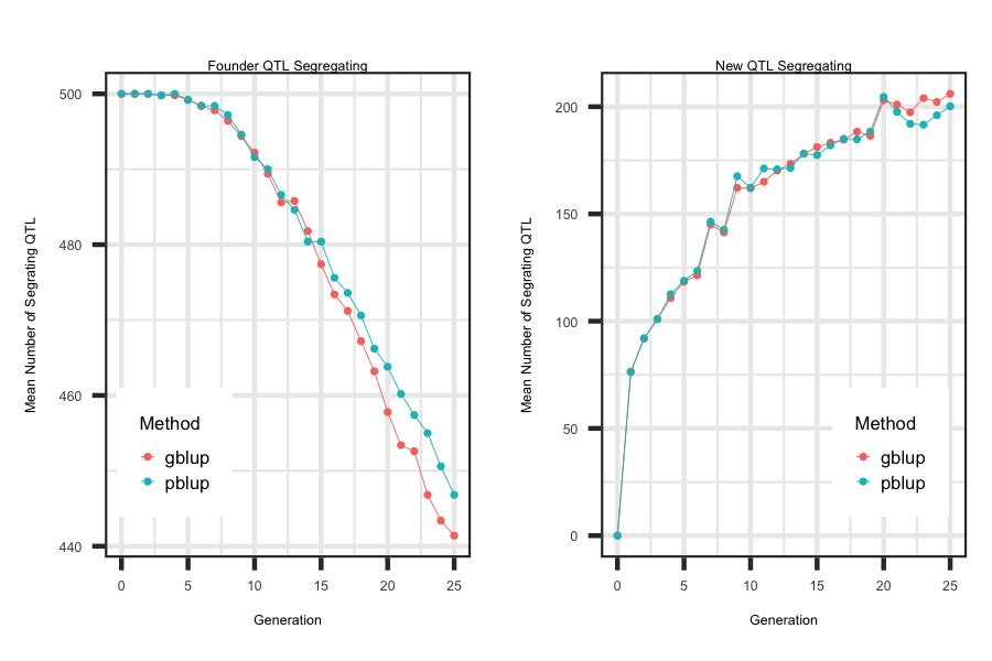
Similar to the previous examples, a bash script is outlined below that illustrates the impact of different ebv prediction on the number of
segregating founder and new mutations by generation. Within each ebv prediction method a simulation that allows new mutations that impact the
quantitative trait is generated. The total number of mutations that are generated within each gamete is sampled from a Poisson distribution with a rate
parameter equal to the mutation rate times the length of the chromosome (i.e. nucleotides). Out of the total mutations that are generated, only
10 percent are assumed to have an effect (i.e. non-neutral) on the quantitative trait. All new mutations are stored in the 'QTL_new_old_Class"
along with the generation they appeared. The two types of prediction methods include pedigree-based or genomic-based BLUP.
Similar to Example 6, the important files are saved within the renamed replicate folder within each scenario. The replicate number is appended to the file name.
Utilizing the R code outlined below the following plot was generated to illustrate how to loop through each scenario and generate plots that describe the impact of the
two ebv prediction methods on the number of founder mutations and new mutations segregating across generations.
R-Code
rm(list=ls()); gc()
library(ggplot2); library(tidyverse)
wd <- "/Users/jeremyhoward/Documents/39_GenoDiver_C++Code/WebsiteExamples/Example18/"
scen <- c("reps_pblup","reps_gblup")
reps <- c(1500:1509)
for(i in 1:length(scen))
{
for(j in 1:length(reps))
{
filename <- paste(wd,scen[i],"/Summary_Statistics_QTL_",reps[j],sep="")
df <- read_table2(file=filename,col_names = TRUE,col_type = "iiiiiiiiidi") %>%
mutate(Method = paste(unlist(strsplit(scen[i],"_"))[2]),
Rep = reps[j]) %>%
select(Generation,Method,Rep,Quant_Founder_Start,Mutation_Quan_Total)
if(j == 1 & i == 1){summarytable <- df}
if(j > 1 | i > 1){summarytable <- rbind(summarytable,df);}
}
}
means <- aggregate(Quant_Founder_Start ~ Generation + Method, data=summarytable,FUN=mean)
sds <- aggregate(Quant_Founder_Start ~ Generation + Method, data=summarytable,FUN=sd)
plotdf <- cbind(means,sds[,3]); rm(means,sds)
names(plotdf) <- c("Generation","Method","Mean","SD")
pd <- position_dodge(0.20)
ggplot(plotdf, aes(x=as.factor(Generation), y=Mean, group=Method, colour=Method)) +
geom_point(size=2.0) + geom_line(size=0.50) + theme_bw() +
labs(title = "Founder QTL Segregating", x = "Generation", y = "Mean Number of Segrating QTL") +
theme(plot.title = element_text(size = 16,hjust = 0.5),axis.title = element_text(size = 12),
legend.position="bottom",axis.text=element_text(size=10))
means <- aggregate(Mutation_Quan_Total ~ Generation + Method, data=summarytable,FUN=mean)
sds <- aggregate(Mutation_Quan_Total ~ Generation + Method, data=summarytable,FUN=sd)
plotdf <- cbind(means,sds[,3]); rm(means,sds)
names(plotdf) <- c("Generation","Method","Mean","SD")
pd <- position_dodge(0.20)
ggplot(plotdf, aes(x=as.factor(Generation), y=Mean, group=Method, colour=Method)) +
geom_point(size=2.0) + geom_line(size=0.50) + theme_bw() +
labs(title = "New QTL Segregating", x = "Generation", y = "Mean Number of Segrating QTL") +
theme(plot.title = element_text(size = 16,hjust = 0.5),axis.title = element_text(size = 12),
legend.position="bottom",axis.text=element_text(size=10))


