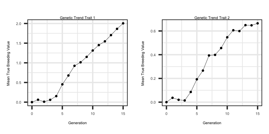
The parameter file outlined below illustrates how to simulate a population undergoing direct selection for a trait along with indirect selection for a genetically
correlated trait. In this scenario two traits are simulated with a correlation of 0.40 and 0.15 for the additive genetic and residual environmental effects between trait 1
and trait 2. If two traits are being simulated and selection is based on 'ebv', by default, the first trait is the one being directly selected and the second trait is
undergoing indirect selection.
−−−−−−−| Running the Program Example |−−−−−−−
−| General |−
START: founder
SEED: 1500
−| Genome & Marker |−
CHR: 3
CHR_LENGTH: 150 150 150
NUM_MARK: 4000 4000 4000
QTL: 150 150 150
−| Population |−
FOUNDER_Effective_Size: Ne70
MALE_FEMALE_FOUNDER: 50 400 random 3
VARIANCE_A: 0.35 0.40 0.35
VARIANCE_R: 0.65 0.15 0.65
−| Selection |−
GENERATIONS: 15
INDIVIDUALS: 50 0.2 400 0.2
PROGENY: 1
SELECTION: ebv high
EBV_METHOD: pblup
CULLING: ebv 5
-| Mating |-
MATING: random125 simu_anneal
Utilizing the R code outlined below the following plots were generated from the output files to see the correlated response in the second trait due to direct selection
on trait one.
R-Code
rm(list = ls()); gc()
library(ggplot2); library(tidyverse)
setwd("/Users/jeremyhoward/Desktop/C++Code/18_GenoDiver_V3/GenoDiverFiles/")
df <- read_table2(file="Summary_Statistics_DataFrame_Performance",col_names = TRUE,col_type = "dcccccccccccc") %>%
mutate(tbv1 = as.numeric(matrix(unlist(strsplit(tbv1, "[()]")), ncol = 2, byrow = TRUE)[, 1]),
tbv2 = as.numeric(matrix(unlist(strsplit(tbv2, "[()]")), ncol = 2, byrow = TRUE)[, 1])) %>%
select(Generation,tbv1,tbv2)
ggplot(df, aes(x = Generation, y = tbv1)) + geom_line(size = 1) + ggtitle("Genetic Trend Trait 1") + theme_bw() +
theme(plot.title = element_text(hjust = 0.5)) + ylab("Mean True Breeding Value ")
ggplot(df, aes(x = Generation, y = tbv2)) + geom_line(size = 1) + ggtitle("Genetic Trend Trait 2") + theme_bw() +
theme(plot.title = element_text(hjust = 0.5)) + ylab("Mean True Breeding Value ")


