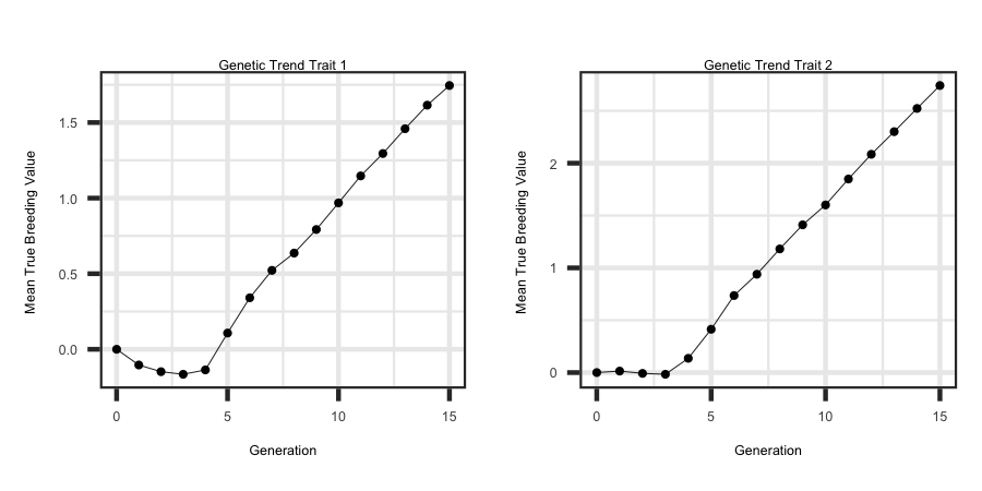
The parameter file outlined below illustrates how to simulate a population undergoing selection based on an index value, which is comprised of the TBV for trait 1 and 2.
The weight in the final index for trait 1 and 2 is 0.25 and 0.75, respectively. In order to make each trait have the same variance, each value is scaled by the standard deviation
in the true breeding values for individuals born in the generation prior to when selection begins (e.g. Generation 3). The index for animal `i' is calculated as follows:
−−−−−−−| Running the Program Example |−−−−−−−
−| General |−
START: founder
SEED: 1500
−| Genome & Marker |−
CHR: 3
CHR_LENGTH: 150 150 150
NUM_MARK: 4000 4000 4000
QTL: 150 150 150
−| Population |−
FOUNDER_Effective_Size: Ne70
MALE_FEMALE_FOUNDER: 50 400 random 3
VARIANCE_A: 0.35 0.40 0.35
−| Selection |−
GENERATIONS: 15
INDIVIDUALS: 50 0.2 400 0.2
PROGENY: 1
SELECTION: index_tbv high
INDEX_PROPORTIONS: 0.25 0.75
CULLING: index_tbv 5
-| Mating |-
MATING: random125 simu_anneal
Utilizing the R code outlined below the following plots were generated from the output files to see the response across both traits.
R-Code
rm(list = ls()); gc()
library(ggplot2); library(tidyverse)
setwd("/Users/jeremyhoward/Desktop/C++Code/18_GenoDiver_V3/GenoDiverFiles/")
df <- read_table2(file="Summary_Statistics_DataFrame_Performance",col_names = TRUE,col_type = "dccccccccccccc") %>%
mutate(tbv1 = as.numeric(matrix(unlist(strsplit(tbv1, "[()]")), ncol = 2, byrow = TRUE)[, 1]),
tbv2 = as.numeric(matrix(unlist(strsplit(tbv2, "[()]")), ncol = 2, byrow = TRUE)[, 1])) %>%
select(Generation,tbv1,tbv2)
ggplot(df, aes(x = Generation, y = tbv1)) + geom_line(size = 1) + ggtitle("Genetic Trend Trait 1") + theme_bw() +
theme(plot.title = element_text(hjust = 0.5)) + ylab("Mean True Breeding Value ")
ggplot(df, aes(x = Generation, y = tbv2)) + geom_line(size = 1) + ggtitle("Genetic Trend Trait 2") + theme_bw() +
theme(plot.title = element_text(hjust = 0.5)) + ylab("Mean True Breeding Value ")


