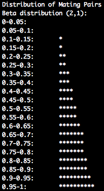
The parameter file outlined below illustrates how to simulate a population where older animals are assigned a larger number of mating
pairs, compared to younger animals. This type of scenario is generated by utilizing the "PARITY_MATES_DIST" parameter with the following values
"2.0 1.0". These two values are utilized to generate the distribution of mating pairs. A Beta distribution, which is parameterized by two parameters,
is used to generate the distribution of mating pairs. A beta distribution was utilized in order to allow for a wide range of mating scenarios. For
example, to generate a scenario where younger animals are assigned a larger number of mating pairs compared to older animals, the parameters need to
be changed to "1.0 2.0". The number of mating pairs by age class are generated by splitting the cumulative distribution function (CDF) into quadrants
based on the number of age classes that occur within a generation. The total number of mating pairs within an age class is the proportion that falls
within the CDF quadrant for a given age class.
−−−−−−−| Differential Sire Contribution by Age |−−−−−−−
−| General |−
START: sequence
SEED: 1501
−| Genome & Marker |−
CHR: 3
CHR_LENGTH: 150 150 150
NUM_MARK: 4000 4000 4000
QTL: 150 150 150
−| Population |−
FOUNDER_Effective_Size: Ne70
MALE_FEMALE_FOUNDER: 50 400 random 3
VARIANCE_A: 0.35
−| Selection |−
GENERATIONS: 15
INDIVIDUALS: 50 0.2 400 0.2
PROGENY: 1
PARITY_MATES_DIST: 2.0 1.0
SELECTION: ebv high
EBV_METHOD: pblup
CULLING: ebv 5
-| Mating |-
MATING: random125 simu_anneal
Once the program has finished, inspection of the log file will provide details on the impact of the "PARITY_MATES_DIST" option. Within the log file
(lines 148-169), the mating distribution CDF is illustrated and is outlined below. When generating the number of matings for a given age class for each
generation the CDF outlined below is split into quadrants based on the number of age classes that occur within a generation. Lastly, the number of matings
within each age class is also outlined in the logfile for each generation.
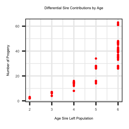
A potential reason for putting this into a simulation is to generate some sires with a large number of progeny, while other sires have
very few progeny. The sires that generate a large number of progeny would then have a large impact on the genome of future generations which may include the
spread of a lethal/sublethal mutation that the sire(s) carry.
Utilizing the R code outlined below the following plot was generated to show the non-linear relationship of number of progeny left by a sire across
different ages that a sire left the herd.
R-Code
rm(list=ls()); gc()
library(ggplot2); library(tidyverse)
setwd("/Users/jeremyhoward/Desktop/C++Code/18_GenoDiver_V3/GenoDiverFiles/")
df <- read_table2(file="Master_DataFrame",col_names = TRUE,col_type = "iiiiiiiidddddiiiiddddddddddd") %>%
filter(.,Progeny > 0) %>%
filter(.,Sex == 0) %>%
filter(.,Gen > 3)
ggplot(df, aes(x=Age, y = Progeny)) + geom_point(colour = "red", size = 3) + xlab("Age Sire Left Population") +
ylab("Number of Progeny") + ggtitle("Differential Sire Contributions by Age") + theme_bw()


